Introduction
![]()
In team sports, the term home advantage – also called home ground, home field, home-field advantage, home court, home-court advantage, defender’s advantage or home-ice advantage – describes the benefit that the home team is said to gain over the visiting team. This benefit has been attributed to psychological effects supporting fans have on the competitors or referees; to psychological or physiological advantages of playing near home in familiar situations; to the disadvantages away teams suffer from changing time zones or climates, or from the rigors of travel; … In baseball, in particular, the difference may also be the result of the home team having been assembled to take advantage of the idiosyncrasies of the home ballpark, such as the distances to the outfield walls; most other sports are played in standardized venues. From Wikipedia - Home advantage
In this post, we will also talk about the competition between the Braves and the Yankees. The table below shows the two possible schedules for each game of the series. (NYC = New York City, ATL = Atlanta)
| Overall advantage | Game 1 | Game 2 | Game 3 | Game 4 | Game 5 | Game 6 | Game 7 |
|---|---|---|---|---|---|---|---|
| Braves | ATL | ATL | NYC | NYC | NYC | ATL | ATL |
| Yankees | NYC | NYC | ATL | ATL | ATL | NYC | NYC |
Let PB be the probability that the Braves win a single head-to-head match-up with the Yankees, under the assumption that home-field advantage does not exist. Let PBH denote the probability that the Braves win a single head-to-head match-up with the Yankees as the home team (H for home). Let PBA denote the probability that the Braves win a single head-to-head match-up as the away team (A for away).
| Game location | No advantage | Advantage |
|---|---|---|
| ATL | PB | PBH = PB $\times$ 1.1 |
| NYC | PB | PBA = 1 - (1 - PB)$\times$ 1.1 |
library(dplyr)
library(data.table)
Now let’s look at the questions.
Questions
1. Compute analytically the probability that the Braves win the World Series when the sequence of game locations is {NYC, NYC, ATL, ATL, ATL, NYC, NYC}. Calculate the probability with and without home-field advantage when PB = 0.55. What is the difference in probabilities?
First, load the .csv file that contains the possible outcomes we need to calculate. This represents the data we will generate later.
# Get all possible outcomes
apo <- fread("all-possible-world-series-outcomes.csv")
We also need to define a sequence of game locations. This time, the sequence should be {NYC, NYC, ATL, ATL, ATL, NYC, NYC}. Since the Braves are based in Atlanta, we use 1 to represent Atlanta and 0 to represent NYC.
# Home field indicator
hfi <- c(0,0,1,1,1,0,0) #{NYC, NYC, ATL, ATL, ATL, NYC, NYC}
Now we use 0.55 to define PB and generate the other probabilities from PB as described above.
# P_B
pb <- 0.55
advantage_multiplier <- 1.1 # Set = 1 for no advantage
pbh <- pb * advantage_multiplier
pba <- 1 - (1 - pb) * advantage_multiplier
In this part, we use the parameters defined above. In every row of the data.table, we use the probabilities influenced by home-field advantage to calculate the overall probability of each situation.
# Calculate the probability of each possible outcome
apo[, p := NA_real_] # Initialize new column in apo to store prob
for(i in 1:nrow(apo)){
  prob_game <- rep(1, 7)
  for(j in 1:7){
    p_win <- ifelse(hfi[j], pbh, pba)
    prob_game[j] <- case_when(
        apo[i,j,with=FALSE] == "W" ~ p_win
      , apo[i,j,with=FALSE] == "L" ~ 1 - p_win
      , TRUE ~ 1
    )
  }
  apo[i, p := prod(prob_game)] # Data.table syntax
}
Then we output the probability that the Braves win the World Series with home-field advantage.
# Probability of overall World Series outcomes
p_home <- purrr::flatten_dbl(apo[, sum(p), overall_outcome][1,2])
p_home
The probability is r p_home.
Then we can calculate the probability when there is no home field advantage.
p_nohome <- 1 - pbinom(3, 7, 0.55)
p_nohome
The probability is r p_nohome. When home-field advantage exists, the probability that the Braves win the World Series is lower, r p_home, than the probability without home-field advantage. Given PB=0.55, the difference between the probability of the Braves winning the World Series with home-field advantage and without home-field advantage is r (p_home-p_nohome)*100 percentage points.
2. Calculate the same probabilities as the previous question by simulation.
In this part, we will use simulation to test the probability.
Given the location sequence, we use different winning probabilities for the head-to-head games and randomly generate the result of each game. By repeating this process 100,000 times, we can approximate the probability with home-field advantage.
set.seed(314)
sml_list_h <- rep(NA, 100000)
for (i in seq_along(sml_list_h)){
  round <- rep(NA,7)
  for(j in 1:7){
    p_win <- ifelse(hfi[j], pbh, pba)
    round[j] <- rbinom(1,1,p_win)
  }
  sml_list_h[i] <- ifelse(sum(round)>=4, 1, 0)
}
mean_sml_h <- mean(sml_list_h)
mean_sml_h
Now we can get the approximate solution, r mean_sml_h, which is a little different from r p_home.
Now, let’s simulate the situation without home-field advantage. This is easy because we only need to set p_win to a constant value.
set.seed(314)
sml_list_nh <- rep(NA, 100000)
for (i in seq_along(sml_list_nh)){
  round <- rep(NA,7)
  for(j in 1:7){
    p_win <- 0.55
    round[j] <- rbinom(1,1,p_win)
  }
  sml_list_nh[i] <- ifelse(sum(round)>=4, 1, 0)
}
mean_sml_nh <- mean(sml_list_nh)
mean_sml_nh
3. What is the absolute and relative error for your simulation in the previous question?
Absolute error = \(|p̂−p|\)
Relative error = \(|p̂−p|/p\).
abs_error_h <- abs(mean(sml_list_h) - p_home)
rel_error_h <- abs(mean(sml_list_h) - p_home)/mean(sml_list_h)
abs_error_h
rel_error_h
Therefore, given home-field advantage the absolute error is r abs_error_h. The relative error is r rel_error_h.
abs_error_nh <- abs(mean(sml_list_nh) - p_nohome)
rel_error_nh <- abs(mean(sml_list_nh) - p_nohome)/mean(sml_list_nh)
abs_error_nh
rel_error_nh
Therefore, given no home-field advantage the absolute error is r abs_error_nh. The relative error is r rel_error_nh.
Bonus 1. Does the difference in probabilities (with vs without home-field advantage) depend on PB?
The process is similar to the answer of question 1.
We can create some lists to save the different PB values, the probabilities of winning the World Series with or without home-field advantage, and the difference between these two situations for different PB values.
Then given every PB, calculate these values every time.
pb_list <- seq(0,1,0.01)
ph_win_list <- seq_along(pb_list)
pnh_win_list <- ph_win_list
diff_list <- ph_win_list
for (p in seq_along(pb_list)) {
  pb <- pb_list[p]
  advantage_multiplier <- 1.1
  pbh <- pb * advantage_multiplier
  pba <- 1 - (1 - pb) * advantage_multiplier

  pnh_win_list[p] <- 1 - pbinom(3, 7, pb_list[p])

  # Calculate the probability of each possible outcome
  apo[, p := NA_real_] # Initialize new column in apo to store prob
  for(i in 1:nrow(apo)){
    prob_game <- rep(1, 7)
    for(j in 1:7){
      p_win <- ifelse(hfi[j], pbh, pba)
      prob_game[j] <- case_when(
          apo[i,j,with=FALSE] == "W" ~ p_win
        , apo[i,j,with=FALSE] == "L" ~ 1 - p_win
        , TRUE ~ 1
      )
    }
  apo[i, p := prod(prob_game)] # Data.table syntax
  }
  ph_win_list[p] <- purrr::flatten_dbl(apo[, sum(p), overall_outcome][1][,2])
  diff_list[p] <- pnh_win_list[p] - ph_win_list[p]
}
Then, plot a graph to show the relationship between PB and differences.
plot(x= pb_list, y=diff_list)
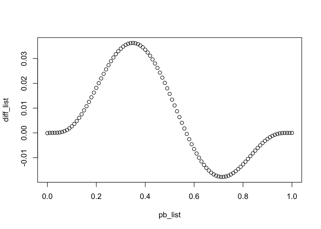
The relationship between PB and the difference appears to resemble a compound function involving trigonometric functions.
The format might be a trigonometric function multiplied by another function that approaches 0 at the beginning and end of one period, and otherwise approaches 1. The period should be 1.
There are some examples. \(y = A \cdot sin(B \cdot x + C) \\ y = A \cdot sin(B \cdot x + C) \cdot |D \cdot sin(\pi \cdot x + E)| \\ y = A \cdot sin(B \cdot x + C) \cdot ( D \cdot sin(\pi \cdot x + E))^2 \\ y = Ax^3 + Bx^2y + Cxy^2+Dy^3 +Ex^2+Fxy+Gy^2+Hx+Iy+J\) Unfortunately, none of the listed functions can fit the graph well.
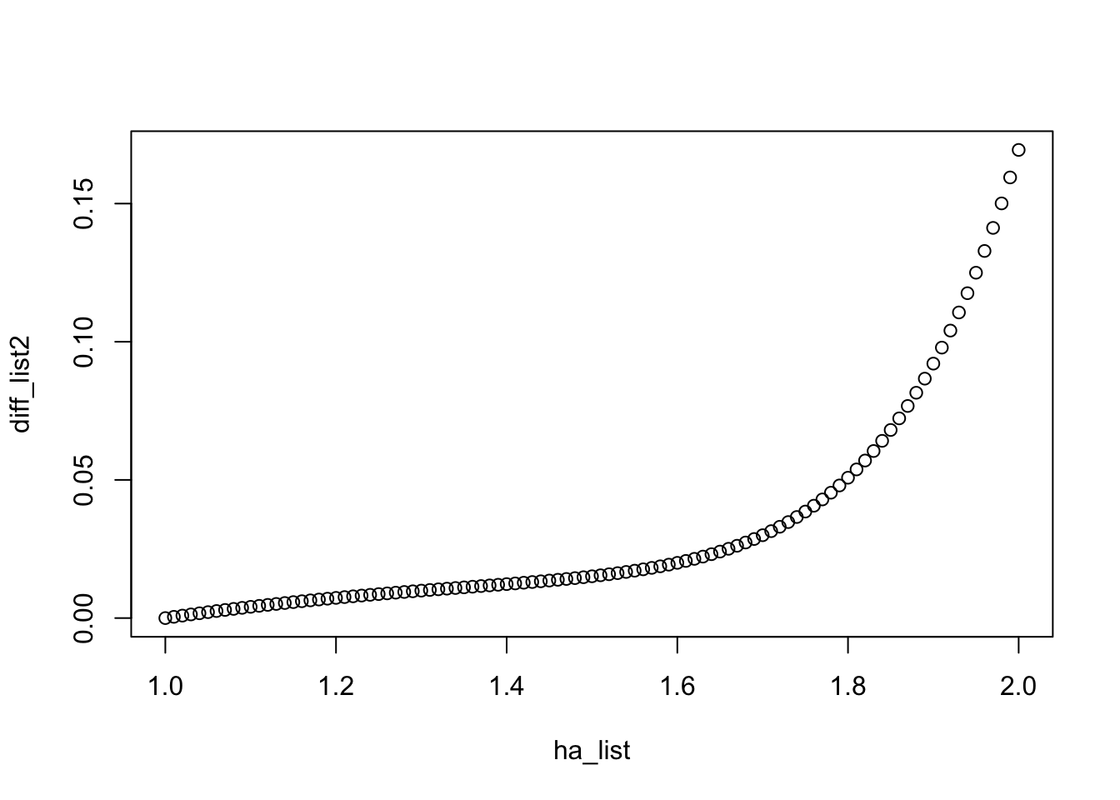
Bonus 2. Does the difference in probabilities (with vs without home-field advantage) depend on the advantage factor? (The advantage factor in PBH and PBA is the 1.1 multiplier that results in a 10% increase for the home team.)
In this question, the process is similar to Bonus 1. We only need to change the sequence values from PB to the home-field advantage factor and set PB as a constant (0.55). Therefore, we will use ha_list to save the sequence.
ha_list <- seq(1,2,0.01)
ph_win_list <- seq_along(ha_list)
pnh_win_list <- ph_win_list
diff_list2 <- ph_win_list
for (p in seq_along(ha_list)) {
  pb <- 0.55
  advantage_multiplier <- ha_list[p]
  pbh <- pb * advantage_multiplier
  pba <- 1 - (1 - pb) * advantage_multiplier

  pnh_win_list[p] <- 1 - pbinom(3, 7, 0.55)

  # Calculate the probability of each possible outcome
  apo[, p := NA_real_] # Initialize new column in apo to store prob
  for(i in 1:nrow(apo)){
    prob_game <- rep(1, 7)
    for(j in 1:7){
      p_win <- ifelse(hfi[j], pbh, pba)
      prob_game[j] <- case_when(
          apo[i,j,with=FALSE] == "W" ~ p_win
        , apo[i,j,with=FALSE] == "L" ~ 1 - p_win
        , TRUE ~ 1
      )
    }
  apo[i, p := prod(prob_game)] # Data.table syntax
  }
  ph_win_list[p] <- purrr::flatten_dbl(apo[, sum(p), overall_outcome][1][,2])
  diff_list2[p] <- pnh_win_list[p] - ph_win_list[p]
}
Let’s look at the graph. When the home-field advantage factor increases, the difference in probabilities between the with- and without-home-field-advantage scenarios also increases.
plot(x= ha_list, y=diff_list2)