Background
Roulette is a casino game named after the French word meaning little wheel. In the game, players may choose to place bets on either a single number, various groupings of numbers, the colors red or black, whether the number is odd or even, or if the numbers are high (19–36) or low (1–18). From Wikipedia-Roulette
In this post, we will look at a simplified version of roulette. Instead of modeling each number on the wheel, we divide each play into only two outcomes: win or lose.
To play the game safely and avoid unrealistic debt, we first need to set several parameters. These parameters will be stored in a state list.
| Parameter | Type | Explanation |
|---|---|---|
| B | number | the budget |
| W | number | the budget threshold for stopping successfully |
| L | number | the maximum number of plays |
| M | number | the casino wager limit |
| plays | integer | the number of plays executed |
| previous_wager | number | the wager in the previous play (0 at first play) |
| previous_win | TRUE/FALSE | indicator of whether the previous play was a win (TRUE at first play) |
Function Setup
One Play
To use the %>% pipe in the code, we need to import the package first.
library(dplyr)
Then, let’s define the process of one play.
 one_play <- function(state){

    # Wager
    proposed_wager <- ifelse(state$previous_win, 1, 2*state$previous_wager)
    wager <- min(proposed_wager, state$M, state$B)

    # Spin of the wheel
    red <- rbinom(1,1,18/38)

    # Update state
    state$plays <- state$plays + 1
    state$previous_wager <- wager
    if(red){
      # WIN
      state$B <- state$B + wager
      state$previous_win <- TRUE
    }else{
      # LOSE
      state$B <- state$B - wager
      state$previous_win <- FALSE
    }
  state
}
When the player runs out of money, wins enough money, or reaches the play limit, we need to stop the game with a stop function.
stop_play <- function(state){
  if(state$B <= 0) return(TRUE)
  if(state$plays >= state$L) return(TRUE)
  if(state$B >= state$W) return(TRUE)
  FALSE
}
Multiple Plays
Next, we simulate the game under these rules as a series of plays. The function returns a budget vector that records the balance after each play.
one_series <- function(
    B = 200
  , W = 300
  , L = 1000
  , M = 100
){

  # initial state
  state <- list(
    B = B
  , W = W
  , L = L
  , M = M
  , plays = 0
  , previous_wager = 0
  , previous_win = TRUE
  )

  # vector to store budget over series of plays
  budget <- rep(NA, L)

  # For loop of plays
  for(i in 1:L){
    new_state <- state %>% one_play
    budget[i] <- new_state$B
    if(new_state %>% stop_play){
      return(budget[1:i])
    }
    state <- new_state
  }
  budget
}
Then we can get the final result of a series of plays.
# helper function
get_last <- function(x) x[length(x)]
get_series <- function(x) x
Simulation
To understand the overall behavior, we need to repeat the process many times and examine the distribution and other characteristics of the results.
# Simulation
walk_out_money <- rep(NA, 1000)
for(j in seq_along(walk_out_money)){
  walk_out_money[j] <- one_series(B = 200, W = 300, L = 1000, M = 100) %>% get_last
}

# Walk out money distribution
hist(walk_out_money, breaks = 100)

# Estimated probability of walking out with extra cash
mean(walk_out_money > 200)

# Estimated earnings
mean(walk_out_money - 200)
Compare
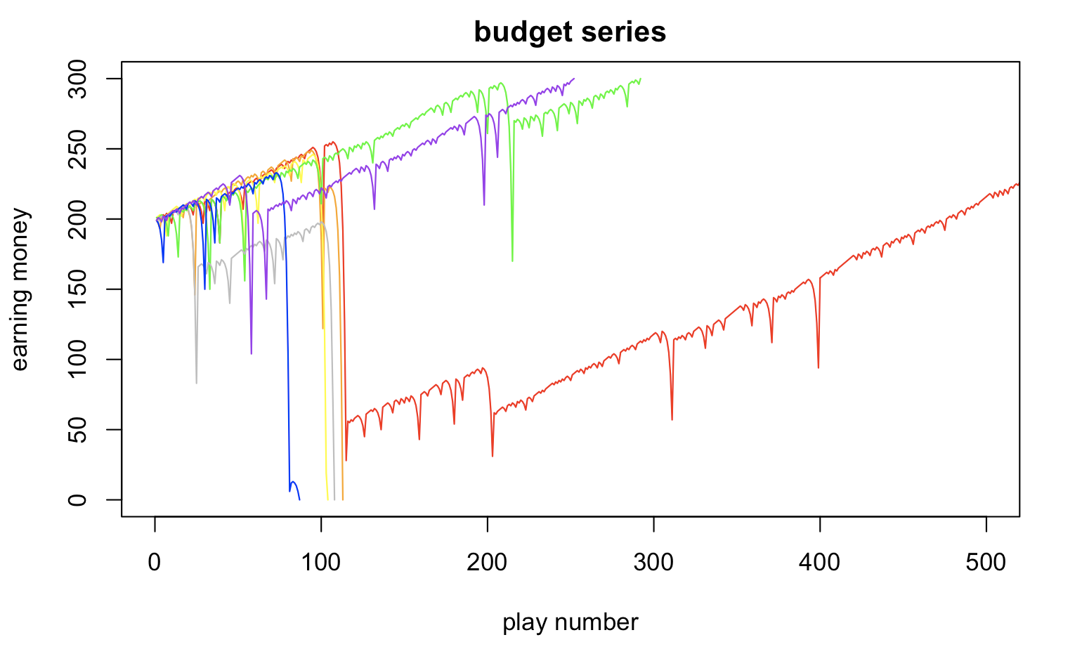
This graph shows how the budget changes during one series.
budget_list <- one_series(B = 200, W = 300, L = 1000, M = 100) %>% get_series
plot(budget_list, type="l", xlim=c(0,500), ylim=c(0,300), xlab="play number", ylab="earning money", main="budget series",col="red")
budget_list <- one_series(B = 200, W = 300, L = 1000, M = 100) %>% get_series
lines(budget_list, col="orange")
budget_list <- one_series(B = 200, W = 300, L = 1000, M = 100) %>% get_series
lines(budget_list, col="yellow")
budget_list <- one_series(B = 200, W = 300, L = 1000, M = 100) %>% get_series
lines(budget_list, col="green")
budget_list <- one_series(B = 200, W = 300, L = 1000, M = 100) %>% get_series
lines(budget_list, col="gray")
budget_list <- one_series(B = 200, W = 300, L = 1000, M = 100) %>% get_series
lines(budget_list, col="blue")
budget_list <- one_series(B = 200, W = 300, L = 1000, M = 100) %>% get_series
lines(budget_list, col="purple")
| Parameter | Type | Explanation |
|---|---|---|
| B | number | the budget |
| W | number | the budget threshold for stopping successfully |
| L | number | the maximum number of plays |
| M | number | the casino wager limit |
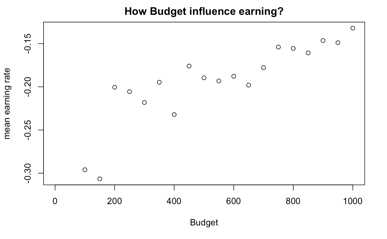
Change the budget
When B changes, what is the mean earning?
earning_series <- rep(NA,20)
for(B in seq(100,1000,by=50)){
walk_out_money <- rep(NA, 1000)
for(j in seq_along(walk_out_money)){
  walk_out_money[j] <- one_series(B, W=B+100, L = 1000, M = 100) %>% get_last
}
earning_series[B] <- mean(walk_out_money - B)/B
}
plot(earning_series,xlab="Budget",ylab="mean earning rate", main="How Budget influence earning?")
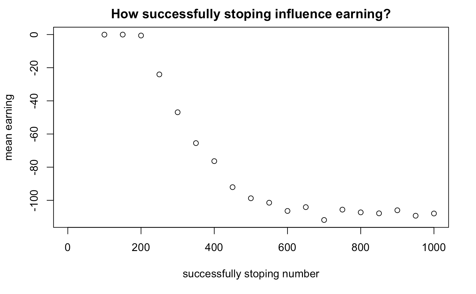
Change the budget threshold for stopping successfully
When W changes, what is the mean earning?
earning_series <- rep(NA,20)
for(W in seq(100,1000,by=50)){
walk_out_money <- rep(NA, 10000)
for(j in seq_along(walk_out_money)){
  walk_out_money[j] <- one_series(B=200, W, L = 1000, M = 100) %>% get_last
}
earning_series[W] <- mean(walk_out_money - 200)
}
plot(earning_series,xlab="successfully stopping threshold",ylab="mean earning", main="How does the stopping threshold influence earnings?")
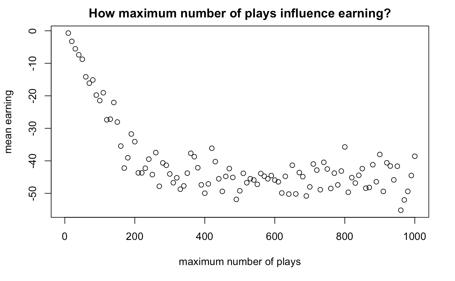
Change the maximum number of plays
When L changes, what is the mean earning?
earning_series <- rep(NA,100)
for(L in seq(10,1000,by=10)){
walk_out_money <- rep(NA, 1000)
for(j in seq_along(walk_out_money)){
  walk_out_money[j] <- one_series(B=200, W=300, L, M = 100) %>% get_last
}
earning_series[L] <- mean(walk_out_money - 200)
}
plot(earning_series,xlab="maximum number of plays",ylab="mean earning", main="How maximum number of plays influence earning?")
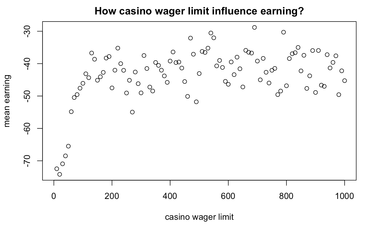
Change the casino wager limit
When M changes, what is the mean earning?
earning_series <- rep(NA,100)
for(M in seq(10,1000,by=10)){
walk_out_money <- rep(NA, 1000)
for(j in seq_along(walk_out_money)){
  walk_out_money[j] <- one_series(B=200, W=300, L=500, M) %>% get_last
}
earning_series[M] <- mean(walk_out_money - 200)
}
plot(earning_series,xlab="casino wager limit",ylab="mean earning", main="How casino wager limit influence earning?")
Play times
Next, we can save the number of plays before the player walks out, then examine its characteristics.
get_times <- function(x) length(x)
walk_out_times <- rep(NA, 10000)
for(j in seq_along(walk_out_times)){
  walk_out_times[j] <- one_series(B = 200, W = 300, L = 1000, M = 100) %>% get_times
}

hist(walk_out_times, breaks = 100)
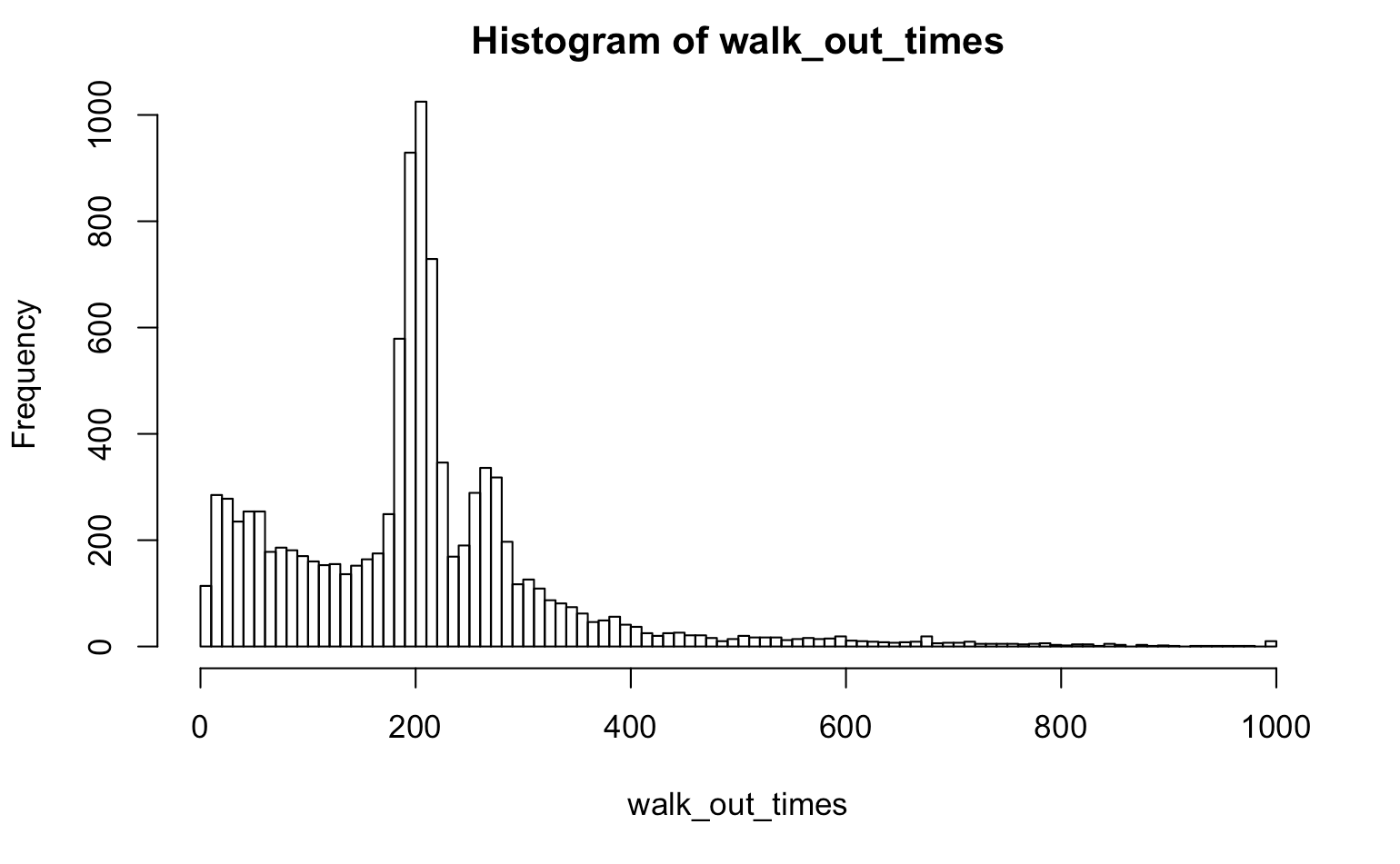
mean(walk_out_times)
The mean number of plays before walking out is 203.0846.
The limitation of simulation is obvious: it is essentially a black box. We cannot use it as a mathematical proof. We do not know exactly why or how the result happened, so we can only change the parameters and try to understand the process. The result is also not perfectly precise; every run will produce a slightly different answer.