Absolute error and relative error are calculated in slightly different ways, but that small difference leads to an important change in interpretation. Absolute error is influenced by sample size, while relative error better reflects the scale of the error itself.
when used as a measure of precision—is the ratio of the absolute error of a measurement to the measurement being taken. In other words, this type of error is relative to the size of the item being measured. RE is expressed as a percentage and has no units.
From Statistics How To
Absolute Error
absolute error = |p̂−p|
The difference between the measured or inferred value of a quantity x_0 and its actual value x.
First, let’s create a table to store the 14*5 simulation results.
n <- rep(NA, 14)
for(i in 1:14){n[i] <- 2^(i+1)}
T <- matrix(NA,14,5)
p <- c(0.01,0.05,0.10,0.25,0.5)
Then we randomly generate 1s and 0s 10,000 times for each setting and calculate the absolute error.
for(x in 1:length(p)){
  for(y in 1:length(n)){
    TS <- rep(NA,10000)
    for(m in 1:10000){
      TS[m] <- abs(rbinom(1,n[y],p[x])/n[y]-p[x])
    }
    T[y,x] <- mean(TS)
  }
}
Change the y-scale to log_10.
T <- log10(T)
Finally, we plot the graph to show the relationship between p and absolute error.
plot(T[,5],xlim=c(0,14),ylim=range(T),col="red",type="b",xaxt="n",xlab="N(log_2 scale)",ylab="Absolute Error",pch=16, lwd=3)
lines(T[,2],col="purple",type="b",pch=16, lwd=3)
lines(T[,3],col="blue",type="b",pch=16, lwd=3)
lines(T[,4],col="green",type="b",pch=16, lwd=3)
lines(T[,1],col="gray",type="b",pch=16, lwd=3)

lname <- c("0.01","0.05","0.10","0.25","0.50")
lname_p <- paste0("p = ",lname)
xname <- c("4","8","16","32","64","128","256","512","1024","2048","4096","8192","16384","32768")

axis(1, at=1:14,las=2, lab=xname)
text(1,T[1,],lname_p,pos=2,cex=0.6)
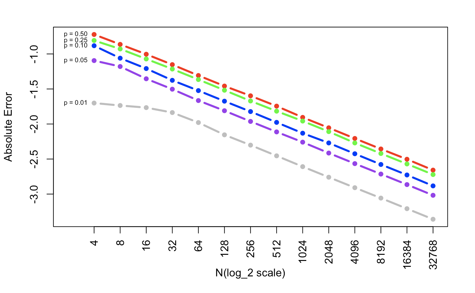
Absolute error is the absolute difference between the observed value and the expected value. In this simulation, we calculate the absolute error 10,000 times and take its mean for each setting. After transforming the y-axis to log_10, it is clear that x and y have a linear relationship. The larger p is, the larger the absolute error becomes.
Relative Error
Relative error = |p̂−p|/p.
Then we do the same thing as before, but when calculating the error, we divide the absolute error by the p-value. We plot this graph as well.
n <- rep(NA, 14)
for(i in 1:14){n[i] <- 2^(i+1)}

T2 <- matrix(NA,14,5)
p <- c(0.01,0.05,0.10,0.25,0.5)

for(x in 1:length(p)){
  for(y in 1:length(n)){
    T2S <- rep(NA,10000)
    for(m in 1:10000){
      T2S[m] <- abs(rbinom(1,n[y],p[x])/n[y]-p[x])/p[x]
    }
    # T2[y,x] <- abs(rbinom(1,n[y],p[x])/n[y]-p[x])/p[x]
    T2[y,x] <- mean(T2S)
  }
}

T2 <- log10(T2)

xname <- c("4","8","16","32","64","128","256","512","1024","2048","4096","8192","16384","32768")
lname <- c("0.01","0.05","0.10","0.25","0.50")
lname_p <- paste0("p = ",lname)

plot(T2[,1],xlim=c(0,14),ylim=range(T2),col="red",type="b",pch=16,xaxt="n",xlab="N(log_2 scale)",ylab="Relative Error", lwd=3)
lines(T2[,2],col="purple",type="b",pch=16, lwd=3)
lines(T2[,3],col="blue",type="b",pch=16, lwd=3)
lines(T2[,4],col="green",type="b",pch=16, lwd=3)
lines(T2[,5],col="gray",type="b",pch=16, lwd=3)
axis(1, at=1:14,las=2, lab=xname)
text(1,T2[1,],lname_p,pos=2,cex=0.6)
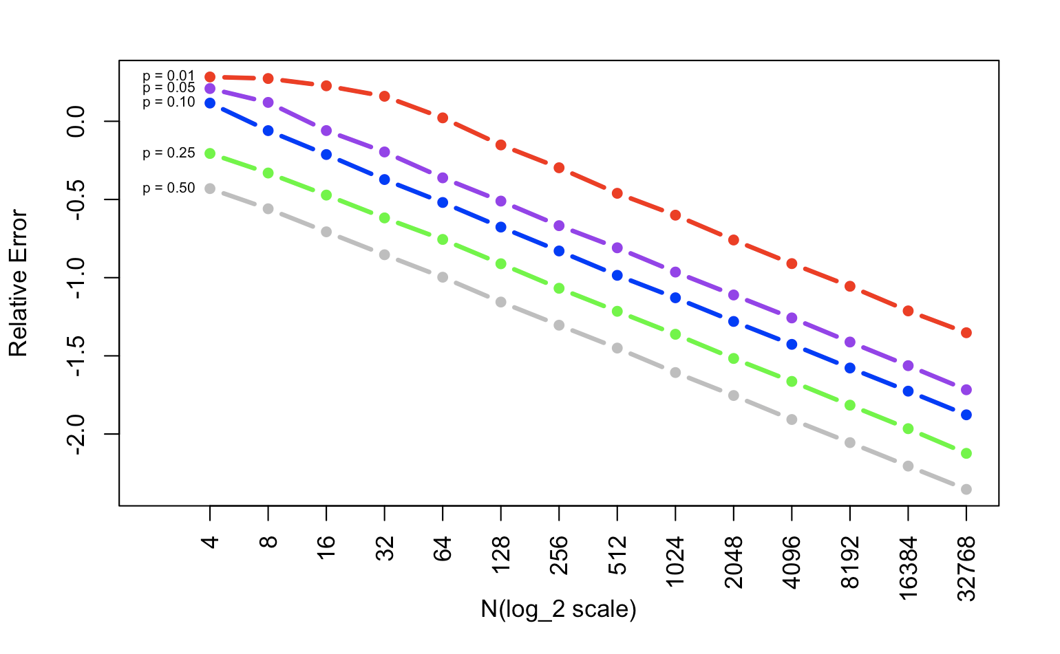
Compared with absolute error, relative error is calculated by dividing the absolute error by p, the expected value. This process accounts for the scale of the value and focuses on the error itself. When we transform the y-axis to log_10, the x-y relationship is also linear. However, the larger p is, the smaller the relative error becomes.